
ELISA 4PL/5PL Standard Curve Fitter – Rigorous Nonlinear Regression for Immunoassay Data
Most ELISA standard curves are still analyzed the wrong way. A sigmoidal dose-response curve gets forced through a straight line, a two-point average, or a spreadsheet trendline — and every concentration calculated from it inherits that error. The ELISA 4PL/5PL Standard Curve Fitter, developed by BioQuant Tools, replaces that guesswork with genuine four-parameter and five-parameter logistic nonlinear regression, solved with a Levenberg–Marquardt optimizer running entirely in your browser.
Enzyme-linked immunosorbent assays (ELISA) are the backbone of cytokine profiling, biomarker validation, and antigen quantification across oncology, immunology, and translational research. Yet the analysis step is frequently the weakest link: Excel cannot fit a true sigmoidal curve, most lab members were never trained on weighted nonlinear regression, and a single mis-fitted standard curve can silently shift every reported concentration in a dataset. This ELISA standard curve calculator was built specifically to close that gap — with the same rigor as GraphPad Prism or SoftMax Pro, accessible directly from any browser, on any device.
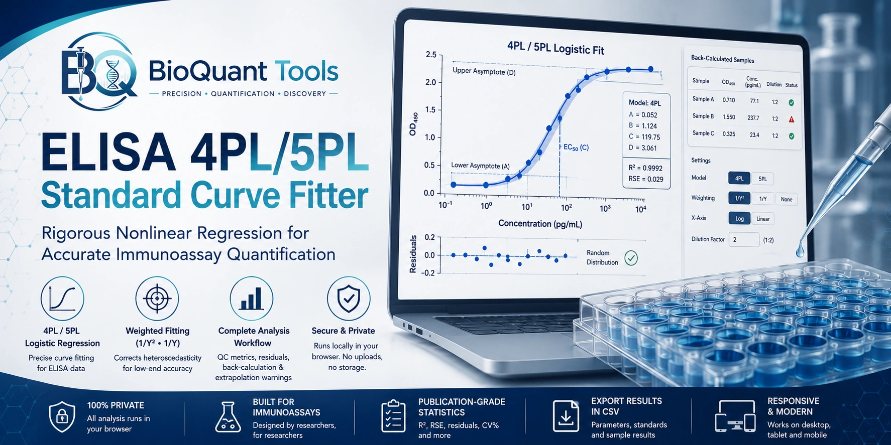
ELISA signal does not increase linearly with concentration — it follows a sigmoidal curve with a defined lower and upper asymptote. Forcing a linear fit through this data systematically overestimates low concentrations and underestimates high ones, exactly where clinical and biological decisions are most sensitive.
ELISA 4PL / 5PL Standard Curve Fitter
Nonlinear logistic regression for immunoassay standard curves — not a linear approximation.
Use 5PL only if the curve is visibly asymmetric near one asymptote; otherwise 4PL is more stable with typical ELISA point counts.
ELISA signal variance grows with response (heteroscedasticity); unweighted fits over-prioritize the top of the curve and distort concentrations at the low end.
Multiplies every back-calculated unknown concentration (e.g. enter 5 for a 1:5 dilution).
Standard Curve Points
Concentration R1 R2 R3 Mean CV%
Dose–Response Curve
Fit Parameters
Goodness of Fit
Residuals Plot
Residuals should scatter randomly around zero. A curved or funnel-shaped pattern signals a poor model choice or that weighting should be changed.
Unknown Samples
Sample Name R1 R2 R3 Mean OD Concentration Flag
This tool runs entirely in your browser — no data is uploaded or stored. Statistical output is a decision-support aid; always apply your own assay validation criteria and scientific judgment before reporting results.
ELISA 4PL / 5PL Standard Curve Fitter
Nonlinear logistic regression for immunoassay standard curves — not a linear approximation.
Use 5PL only if the curve is visibly asymmetric near one asymptote; otherwise 4PL is more stable with typical ELISA point counts.
ELISA signal variance grows with response (heteroscedasticity); unweighted fits over-prioritize the top of the curve and distort concentrations at the low end.
Multiplies every back-calculated unknown concentration (e.g. enter 5 for a 1:5 dilution).
Standard Curve Points
| Concentration | R1 | R2 | R3 | Mean | CV% |
|---|
Dose–Response Curve
Fit Parameters
Goodness of Fit
Residuals Plot
Residuals should scatter randomly around zero. A curved or funnel-shaped pattern signals a poor model choice or that weighting should be changed.
Unknown Samples
| Sample Name | R1 | R2 | R3 | Mean OD | Concentration | Flag |
|---|
This tool runs entirely in your browser — no data is uploaded or stored. Statistical output is a decision-support aid; always apply your own assay validation criteria and scientific judgment before reporting results.
What Does the ELISA 4PL/5PL Standard Curve Fitter Calculate?
This is not a single-number calculator. It is a complete standard-curve analysis workflow, curve fitting, quality control, and sample back-calculation, in one interface.
| Feature | What It Does |
|---|---|
| 4PL / 5PL Model Selection | Fits a symmetric four-parameter logistic curve, or a five-parameter logistic curve for asymmetric dose-response data |
| Levenberg–Marquardt Regression | Solves the nonlinear least-squares problem with data-driven initial parameter estimation for reliable convergence on real, noisy plate data |
| 1/Y and 1/Y² Weighting | Corrects for the heteroscedasticity inherent to immunoassay signal, so accuracy at the low end of the curve is not sacrificed for accuracy at the high end |
| Replicate Mean, SD & %CV | Calculates precision at every standard point and automatically flags high-variability replicates |
| Back-Calculated Sample Concentration | Solves the analytical inverse of the fitted curve to convert unknown sample OD directly into concentration, with dilution factor correction |
| Extrapolation Warning | Flags any sample whose signal falls outside the validated standard curve range before it reaches your report |
| Residuals Plot | Visual diagnostic for detecting a poorly chosen model or weighting scheme |
| R² & Residual Standard Error | Quantitative goodness-of-fit metrics for every curve |
How the ELISA 4PL/5PL Fitter Works
The four-parameter logistic model describes the sigmoidal relationship between analyte concentration (x) and assay response (y):
where A and D are the lower and upper response asymptotes, C is the inflection point (EC50), and B is the Hill slope describing the steepness of the transition. The five-parameter logistic (5PL) model adds an asymmetry factor E, which allows the curve to approach its two asymptotes at different rates, useful when a standard curve visibly bends unevenly near one end.
The tool estimates sensible starting parameters directly from your data, then refines them using the Levenberg–Marquardt algorithm until the (optionally weighted) sum of squared residuals is minimized. Unknown sample concentrations are then recovered using the exact analytical inverse of the fitted equation, not a lookup table or manual interpolation, before the dilution factor is applied.
Key Features of the ELISA 4PL/5PL Standard Curve Fitter
- Symmetric (4PL) and asymmetric (5PL) logistic regression
- 1/Y and 1/Y² weighting for heteroscedastic immunoassay data
- Automatic replicate mean, SD, and %CV with QC flagging
- Analytical back-calculation of unknown concentrations
- Configurable dilution factor correction
- Extrapolation (out-of-range) warnings on every sample
- Interactive dose-response chart with linear or logarithmic X-axis
- Residuals plot for visual fit diagnostics
- R², residual standard error, and convergence status reported for every fit
- One-click CSV export of parameters, standards, and sample results
- Runs 100% client-side — no plate data ever leaves your browser
- Fully responsive on desktop, tablet, and mobile
Real Laboratory Example: Quantifying Serum IL-6 by Sandwich ELISA
A translational oncology lab is quantifying interleukin-6 (IL-6) in patient serum by sandwich ELISA to correlate systemic inflammation with treatment response. An eight-point standard curve is run in duplicate, spanning 0–200 pg/mL:
| Standard (pg/mL) | Mean OD450 |
|---|---|
| 0 | 0.052 |
| 3.13 | 0.098 |
| 6.25 | 0.161 |
| 12.5 | 0.279 |
| 25 | 0.482 |
| 50 | 0.861 |
| 100 | 1.432 |
| 200 | 1.968 |
Fitting this data with a 1/Y²-weighted 4PL model converges in 7 iterations and returns:
- A (bottom asymptote) = 0.052
- B (Hill slope) = 1.124
- C (EC50) = 119.75 pg/mL
- D (top asymptote) = 3.061
- R² = 0.9992, residual standard error = 0.029
Two patient serum samples, each diluted 1:2, are then read against this curve:
- Patient A — OD450 = 0.71 → back-calculated concentration = 77.1 pg/mL, comfortably inside the standard curve range.
- Patient B — OD450 = 1.55 → back-calculated concentration = 237.7 pg/mL, which exceeds the top standard (200 pg/mL). The tool automatically raises an extrapolation flag rather than silently reporting a number derived outside the validated curve range.
This is exactly the failure mode that manual Excel-based analysis misses most often: Patient B's result looks plausible in isolation, but reporting it without recognizing it as an extrapolation risks a biased value. The correct next step, diluting Patient B's sample further and re-assaying, is a QC decision the tool prompts automatically instead of leaving it to chance.
Why Researchers Choose BioQuant Tools
The ELISA 4PL/5PL Standard Curve Fitter is part of an integrated ecosystem of molecular and cellular biology calculators built for the way real experiments actually flow from sample prep through quantification.
- Serial Dilution Calculator — design the standard curve dilution series before you run the plate
- Bradford Protein Assay Calculator — quantify total protein input alongside your target analyte
- Western Blot Quantification Tool — orthogonally confirm protein-level findings
- IC50 Calculator — the same nonlinear logistic engine, applied to dose-response and inhibition data
- qPCR Fold Change Calculator Pro — correlate protein-level ELISA results with transcript-level expression
Best Practices for ELISA Standard Curve Analysis
- Run standards and unknowns in at least duplicate; flag any replicate pair with %CV above 15%
- Always include a true zero/blank standard and subtract background where appropriate
- Start with 4PL; move to 5PL only if the curve is visibly asymmetric near one asymptote
- Use 1/Y² weighting by default for standard sandwich ELISA formats
- Never report a concentration back-calculated from a sample signal outside the standard curve's response range
- Re-dilute and re-assay any sample flagged as out-of-range rather than extrapolating
- Inspect the residuals plot, not just R², before trusting a fit
- Keep the standard curve dilution series consistent across plates/runs for longitudinal comparability
External Scientific Resources
For further reading on immunoassay design and nonlinear curve fitting, researchers may consult:
- NCBI
- Thermo Fisher Scientific — ELISA Technical Resources
- R&D Systems (Bio-Techne) — ELISA Technical Guide
- U.S. FDA — Bioanalytical Method Validation Guidance
Frequently Asked Questions (FAQ)
Why shouldn't I just use a linear fit or a trendline in Excel for my ELISA standard curve?
ELISA response is sigmoidal by nature — signal plateaus at both very low and very high concentrations. A linear fit ignores this shape entirely, systematically distorting concentrations at both ends of the curve. Even a "quadratic" or "log-log" trendline in Excel is still a linear regression in disguise; it does not solve for true logistic parameters and cannot correctly weight heteroscedastic data.
When should I use 5PL instead of 4PL?
Use 5PL only when your standard curve shows clear, visible asymmetry near one of its asymptotes that a symmetric 4PL curve cannot capture — this is more common in high-sensitivity assays with a wide dynamic range. With typical 6–8 point ELISA standard curves, 4PL is usually more stable, since 5PL requires an additional free parameter and therefore more data to constrain it reliably.
Why does weighting (1/Y or 1/Y²) matter for ELISA curve fitting?
ELISA signal variance is not constant across the assay range — optical density readings at high concentrations naturally vary more in absolute terms than readings near the blank. An unweighted fit implicitly treats all points as equally precise, which lets the high-concentration standards dominate the regression and degrades accuracy exactly where sensitivity usually matters most: near the lower limit of quantification.
What does it mean when a sample is flagged as "out of range" or "extrapolated"?
It means the sample's signal falls outside the response range spanned by your standards, so calculating a concentration from it requires extrapolating beyond the curve region your standards actually validated. Extrapolated values are not reliable for reporting. The correct response is to dilute the sample further (if the signal is too high) or concentrate/re-assay it (if too low) so it falls within the standard curve.
What replicate %CV is acceptable for ELISA standards and samples?
A %CV below 15% for replicate wells is a widely used acceptability threshold for immunoassays, though individual assay validation protocols may set stricter or more permissive limits. Consistently high CV at specific concentrations often points to pipetting technique, edge effects on the plate, or a standard nearing the assay's limits of detection.
Is R² alone enough to judge whether my ELISA curve fit is good?
No. R² is a useful diagnostic but was originally developed for linear regression; for a nonlinear logistic fit it can look misleadingly high even when the model systematically misses in a particular region of the curve. Always inspect the residuals plot alongside R² — a curved or funnel-shaped pattern in the residuals signals a fitting problem that R² alone will not reveal.
How is the dilution factor applied to my sample concentration?
The tool first back-calculates the concentration corresponding to your sample's mean OD using the inverse of the fitted curve, then multiplies that value by the dilution factor you specify (e.g., 2 for a 1:2 dilution) to report the concentration in the original, undiluted sample.
Does this tool store or upload my plate data?
No. All curve fitting, statistics, and back-calculation run entirely in your browser using JavaScript. No standard curve values, sample data, or results are transmitted to or stored on any server, which matters when working with unpublished research or patient-derived data.
Can I use this tool for assays other than ELISA?
Yes. The underlying 4PL/5PL nonlinear regression engine is the same mathematics used for any sigmoidal dose-response relationship, including other plate-based immunoassays. For inhibition and dose-response pharmacology data specifically, the companion IC50 Calculator applies the same fitting engine to that use case.
Conclusion
The ELISA 4PL/5PL Standard Curve Fitter from BioQuant Tools brings publication-grade nonlinear regression — weighted fitting, replicate QC, analytical back-calculation, and extrapolation safeguards — to a task that is still, far too often, handled with a straight line in a spreadsheet. Whether you are validating a biomarker, profiling cytokines in an oncology cohort, or running routine antigen quantification, this tool gives you the statistical rigor of dedicated bioanalytical software without leaving your browser.
Home | Serial Dilution Calculator | Bradford Protein Assay Calculator | IC50 Calculator | Western Blot Quantification Tool | About Us | Why BioQuant Tools | Contact Us