
Western Blot Quantification Tool Pro
Welcome to the advanced protein analysis suite brought to you by BioQuant Tools. Quantitative immunoblotting remains one of the most widely utilized molecular biology techniques for determining target protein expression across experimental groups. However, turning chemiluminescent or fluorescent band intensity into publication-grade data requires rigorous background subtraction, loading control normalization, fold-change computation, and statistical validation. Our Western Blot Quantification Tool Pro automates these critical mathematical transformations, eliminating manual spreadsheet errors and ensuring your Western blot analysis meets stringent journal peer-review standards.
In modern biomedical research, subtle shifts in target protein translation or degradation can dictate cell fate. Human computational errors during densitometry normalization can easily obscure true biological effects or introduce false-positive differential expression. By leveraging our automated Western Blot Quantification Tool Pro, researchers can standardize their protein expression workflows. For a comprehensive downstream assay workflow, pair this quantification engine with our qPCR fold change calculator pro, paired qPCR calculator, cell seeding calculator, and serial dilution calculator to connect genomic transcription with protein translation seamlessly.
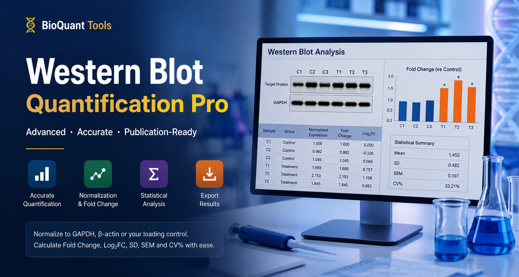
Western Blot Quantification Tool Pro
Advanced protein expression analysis with normalization, fold change calculation and publication-ready outputs.
Experimental Data Input
| Sample | Target Band | Background | Loading Control | Group | Action |
|---|---|---|---|---|---|
Analysis Settings
The Biophysical Fundamentals of Quantitative Immunoblotting
Western blotting transitions from a qualitative presence/absence assay into a quantitative tool when signal intensity linearly correlates with the mass of target protein immobilized on the membrane surface. Achieving high quantitative fidelity depends on three vital biological and optical principles:
- Linear Dynamic Range: Ensuring both target protein and loading control signals fall within the non-saturated detection range of CCD cameras or laser scanners.
- Local Background Signal Subtraction: Removing uniform membrane background autofluorescence or non-specific substrate oxidation noise around each specific band.
- Internal Loading Control Normalization: Adjusting for unavoidable pipetting variations, unequal total protein loading, transfer non-uniformity across gel lanes, and edge artifacts using constitutive housekeeping proteins (e.g., GAPDH, β-Actin, α-Tubulin).
Core Mathematical Formulas & Computational Logic
The Western Blot Quantification Tool Pro processes your raw integrated density values (Densitometry Unit outputs from ImageJ, Image Lab, or Studio Lite) using the standard mathematical steps detailed below:
Subtract the surrounding local background optical density from the raw target band integrated density to yield the net target intensity:
Corrected Target Intensity (Itarget) = Raw Target Intensity - Local Background Target
Corrected Control Intensity (ILC) = Raw Loading Control Intensity - Local Background Control
Divide the net target band intensity by the net internal loading control intensity for every sample lane:
Normalized Relative Ratio (Rnorm) = Itarget / ILC
Calculate the arithmetic mean of normalized relative ratios across all replicates in the baseline reference group (R̄ref). The relative fold change for any individual sample is defined as:
Fold Change (FC) = Rnorm / R̄ref
To normalize log-fold distributions for symmetric representation during statistical modeling and publication plotting, calculate the logarithmic transformation:
log2FC = log2(Fold Change)
For experimental replicates within defined treatment conditions, key parametric statistics summarize inter-lane consistency:
Mean (μ) = (Σ Rnorm) / N
Standard Error of the Mean (SEM) = SD / √N
Percent Coefficient of Variation (CV%) = (SD / μ) × 100
Common Loading Controls in Protein Quantification
Selecting an appropriate housekeeping gene product is essential for accurate normalization. Below is a comparative guide to commonly used internal controls:
| Loading Control Protein | Molecular Weight (kDa) | Subcellular Location | Optimal Biological Application |
|---|---|---|---|
| GAPDH | 36–38 kDa | Cytoplasm | General cellular lysates; high metabolic rate samples. |
| β-Actin | 42 kDa | Cytoskeleton | Whole cell extracts; structural cytoskeletal evaluations. |
| α-Tubulin / β-Tubulin | 50–55 kDa | Cytoskeleton | Neuronal tissues, cell division studies, microtubule assays. |
| Lamin B1 / Fibrillarin | 67 kDa / 34 kDa | Nucleus | Nuclear fraction preparations and chromatin-binding assays. |
| VDAC1 / COX IV | 31 kDa / 17 kDa | Mitochondria | Mitochondrial fractionations and metabolic organelle studies. |
Worked Example: Real-World Research Application
A cancer research laboratory is investigating whether a novel small-molecule inhibitor can suppress PD-L1 protein expression in non-small cell lung cancer (NSCLC) cells. Since PD-L1 is a key immune checkpoint protein involved in tumor immune evasion, reducing its expression may improve anti-tumor immune responses.
Researchers perform a Western blot experiment using the following parameters:
- Target Protein: PD-L1
- Loading Control: GAPDH
- Cell Line: A549 (NSCLC)
- Experimental Groups: Control (Vehicle-treated) vs. Drug Treatment (48 hours)
Raw Densitometry Data (ImageJ Output)
| Sample | Group | PD-L1 Band Intensity | Background | GAPDH Intensity |
|---|---|---|---|---|
| C1 | Control | 15,200 | 1,000 | 18,000 |
| C2 | Control | 14,800 | 1,000 | 17,500 |
| C3 | Control | 15,500 | 1,100 | 18,200 |
| T1 | Treatment | 9,600 | 950 | 17,800 |
| T2 | Treatment | 8,900 | 900 | 17,600 |
| T3 | Treatment | 9,300 | 1,000 | 18,100 |
Step-by-Step Computational Workflow
Step 1: Background Correction
The software first subtracts the background signal (Corrected Intensity = Target Band − Background):
Example (C1): 15,200 − 1,000 = 14,200
Step 2: Normalization to GAPDH
To compensate for loading differences between lanes (Normalized Expression = Corrected Intensity / GAPDH Intensity):
Example (C1): 14,200 / 18,000 = 0.789
Step 3: Calculate Control Mean
Normalized expression values for control samples: C1 = 0.789, C2 = 0.789, C3 = 0.791
Control Mean = 0.790
Step 4: Fold Change & log2FC Analysis
Divide normalized expression of each sample by the control mean (Fold Change = Sample / Control Mean):
Example (T1): 0.486 / 0.790 = 0.615
Quantification Results
| Sample | Group | Normalized Expression | Fold Change | log2FC |
|---|---|---|---|---|
| C1 | Control | 0.789 | 1.000 | 0.000 |
| C2 | Control | 0.789 | 0.999 | -0.001 |
| C3 | Control | 0.791 | 1.002 | 0.003 |
| T1 | Treatment | 0.486 | 0.615 | -0.701 |
| T2 | Treatment | 0.455 | 0.576 | -0.796 |
| T3 | Treatment | 0.458 | 0.580 | -0.786 |
Statistical Summary (Treatment Group)
| Statistical Metric | Calculated Value |
|---|---|
| Mean Expression | 0.628 |
| Standard Deviation (SD) | 0.165 |
| Standard Error (SEM) | 0.067 |
| Coefficient of Variation (CV%) | 26.3% |
Biological Interpretation
The Western blot analysis demonstrates a substantial reduction in PD-L1 protein expression following treatment with the investigational inhibitor. Compared with the control group, treated samples exhibited approximately 40–45% lower PD-L1 expression, with fold-change values ranging from 0.58 to 0.62. Negative log₂ fold-change values further confirm downregulation of PD-L1 at the protein level.
These findings suggest that the compound may suppress immune checkpoint signaling and could potentially enhance anti-tumor immune responses when combined with immunotherapeutic approaches.
Why Use BioQuant Western Blot Quantification Pro?
Instead of manually performing complex calculations in spreadsheets, our online platform automatically:
- Performs precise local background subtraction
- Normalizes target proteins to GAPDH, β-Actin, or Tubulin
- Calculates relative Fold Change and log₂ Fold Change values
- Generates comprehensive statistical summaries (Mean, SD, SEM, CV%)
- Produces publication-ready quantitative outputs and visual bar charts
- Minimizes human calculation errors and maximizes experimental reproducibility
This makes BioQuant Western Blot Quantification Pro an essential tool for researchers working in cancer biology, immunology, molecular biology, cell signaling, drug discovery, and translational medicine.
Step-by-Step Guide to Using Western Blot Quantification Tool Pro
- Enter Experimental Data: Input raw integrated density values for target bands, background region, loading control intensity, and assign group tags (e.g., Control, Treatment A). Click "+ Add Sample" for additional lanes.
- Configure Analysis Settings: Select your internal loading control type (e.g., GAPDH, β-Actin) and identify your baseline Reference Group (e.g., Control).
- Execute Densitometry Analysis: Click Analyze Western Blot to perform background subtraction, normalized ratio calculation, fold change determination, and log2 transformation.
- Review Visualizations & Summary Statistics: Analyze calculated sample metrics including Mean, SD, SEM, and CV%. Inspect auto-generated Fold Change bar charts.
- Export Publication-Ready Data: Click Export CSV to save raw and transformed values directly for submission packages or statistical software processing.
For more details on standard blotting protocols and antibody validations, refer to the NCBI Western Blot Guide.
Frequently Asked Questions (FAQ)
1. Why is background subtraction essential in Western blot densitometry?
Membrane background signals originate from non-specific antibody binding, substrate auto-fluorescence, and detection noise. Subtracting local background ensures that optical density measurements represent target protein mass rather than background artifacts.
2. Should I use Total Protein Normalization (TPN) or Housekeeping Proteins?
Housekeeping proteins (such as GAPDH or β-Actin) are widely accepted for standard normalization. However, Total Protein Normalization (staining membranes with Ponceau S or stain-free technologies) is increasingly favored by top-tier journals when treatment conditions alter housekeeping gene expression or cause protein saturation.
3. What does log2 Fold Change (log2FC) represent, and why is it useful?
The log2FC transformation converts asymmetrical fold changes (where a 2-fold decrease is 0.5 and a 2-fold increase is 2.0) into a symmetric linear scale where 1.0 represents a doubling and -1.0 represents a halving. This simplifies standard parametric statistical comparisons and visualization.
4. How do I know if my band intensities are saturated?
In digital imaging systems, saturated band pixels hit maximum pixel capacity (e.g., 65,535 in 16-bit images), causing image clipping. Saturated bands appear completely flat on peak intensity profiles, underestimating dark bands and invalidating linear quantifications.
5. What CV% range is considered acceptable for biological replicates in immunoblotting?
An intra-assay Coefficient of Variation (CV%) under 10–15% reflects robust technical handling and clean protein transfer. Higher CV% values usually point to uneven gel transfer, inconsistent pipetting, or non-linear chemiluminescent antibody kinetics.